from ngsolve import *
from ngsolve.webgui import Draw
from ngsolve.meshes import *
import matplotlib.pyplot as plt


### Macro Meshing ###
k = 1 # Order of elements
Ne = 212 # Number of elements

### Deterministic Meshing ###
Ne_deterministic = 10000

### Micro Meshing ###
Ne_m = 75
lm = 5e-3

### Physical ###
U = 2
eta = 1e-1
rho = 1
h0 = 0.2
dhdx = 0.15

# Microscale roughness
Ah = 10e-3

# Coupling tolerance
p_tol = 1e-6

# Newton solver tolerance (macro and micro)
Newton_tol = 1e-61D lubrication HMM: the Reynolds equation across scales
HMM
lubrication
Reynolds equation
NGSolve
The Heterogeneous Multiscale Method applied to a 1D lubrication film: the steady, isoviscous, Newtonian Reynolds equation solved as a smooth macro baseline, a fine-resolved textured reference, and an HMM coupling whose micro cell problems supply effective coefficients to a coarse macro solve. Implemented in NGSolve.
This is the lubrication counterpart to the generic 1D HMM demo: the same multiscale machinery, but applied to a thin-film bearing rather than a generic elliptic problem. We solve the steady, isoviscous, Newtonian Reynolds equation in flux-conservation form,
\[ \nabla\cdot(\rho\,q) = 0, \qquad q = \frac{U\,H(x)}{2} \;-\; \frac{H^{3}(x)}{12\,\eta}\,\nabla P, \]
where \(H(x)\) is the film thickness, \(U\) the entrainment speed, \(\eta\) the viscosity and \(P\) the pressure — the Couette (shear-driven) and Poiseuille (pressure-driven) contributions to the flux \(q\). As in the elliptic demo, three scenarios are compared: a smooth macro solve using only the large-scale film shape; a deterministic solve that resolves the full textured film on a fine mesh; and the HMM solve, where micro cell problems over a representative patch of texture feed an effective flux relation back to a coarse macro solve. The finite-element solves use NGSolve.
TipRunning it yourself
Colab is the route to use here — the notebook’s first cell installs NGSolve automatically (via fem-on-colab) on a real cloud kernel.
One dependency to wire up first: the notebook imports a local helper module with from plot_funcs import *. Opening the notebook in Colab loads only the .ipynb, not the rest of the repo, so that import will fail until plot_funcs.py is made available — either by adding a setup cell that fetches it (!wget <raw-github-url>/plot_funcs.py) or by pasting its contents into the notebook. (Binder isn’t offered for this one: the repo’s shared Binder environment targets the FEniCS notebooks, whereas this one self-installs NGSolve on Colab.)
The full notebook is embedded below (install cell and console logs trimmed for reading; the runnable version is linked above).
Parameters and initialisation of macroscale finite element spaces
Macroscale Solver
Solving the smooth, steady, isoviscous, newtonian 1D Lubrication problem.
We can define the problem as being conservation of flux.
Strong form:
\[ \nabla \cdot \rho q = 0 \\ q = \frac{UH(x)}{2} - \frac{H^3(x)}{12 \eta}\nabla P \]
- Weak form/Lagrangian
- BCs
from ngsolve.solvers import *
import numpy as np
from ngsolve.webgui import Draw

def Solve_Macroscale(mesh, hg, dQ, dP):

  # Create a H1, order k space for the pressure field
  V_Macro = H1(mesh, order=k, dirichlet=".*") # All boundaries are set to dirichlet, p = 0. Neumann conditions applied naturally in the weak form.
  p = V_Macro.TrialFunction()  # Pressure trial function
  v = V_Macro.TestFunction()   # Pressure test function
  p_Macro = GridFunction(V_Macro)  # solution
  film_Macro = GridFunction(V_Macro)
  dpdx_Macro = GridFunction(V_Macro)

  a_Macro = BilinearForm(V_Macro)
  h = hg(x, h0, dhdx)
  a_Macro += (h**3 / (12 * eta)) * grad(p) * grad(v) * dx - (U/2) * h * grad(v) * dx
  if dQ is not None:
    dQ_gf = GridFunction(V_Macro)
    dQ_gf.vec.FV().NumPy()[:] = dQ  # load nodal values
    a_Macro += -dQ_gf * grad(v) * dx
  a_Macro.Assemble()

  Newton(
      a_Macro,
      p_Macro,
      freedofs=V_Macro.FreeDofs(),
      maxit=100,
      maxerr=Newton_tol,
      inverse="sparsecholesky",
      printing=False,
  )
  film_Macro.Set(h)
  dpdx = grad(p_Macro)
  dpdx_Macro.Set(dpdx)

  #Construct array of zeta: {H, P, dPdX}
  zeta = np.array([film_Macro.vec.data, p_Macro.vec.data, dpdx_Macro.vec.data])
  return zeta

def q_re(zeta_i):
  """
  Helper function for calculating nodal flux per Reynolds
  """
  H, P, dPdX = zeta_i
  return U * H/2 - H**3 * dPdX / (12 * eta)
Solve Macroscale Smooth
# Film thickness function
def hg(x, h0, dhdx):
  return h0 - dhdx*x

# Create mesh
mesh = Make1DMesh(Ne)

# Solve
zeta = Solve_Macroscale(mesh, hg, 0, 0)
Q_re_smooth = q_re(zeta)
zeta_smooth = zeta
Deterministic
# Create Determinstic mesh
mesh_deterministic = Make1DMesh(Ne_deterministic)

def hg_determinstic(x, h0, dhdx):
  return h0 - dhdx*x + Ah * cos(2 * pi * x/lm)
import time
start = time.time()
zeta_deterministic = Solve_Macroscale(mesh_deterministic, hg_determinstic, 0, 0)
print(f'Exec time {time.time() - start}')
from plot_funcs import *
plot_zeta_combined(zeta, zeta_deterministic)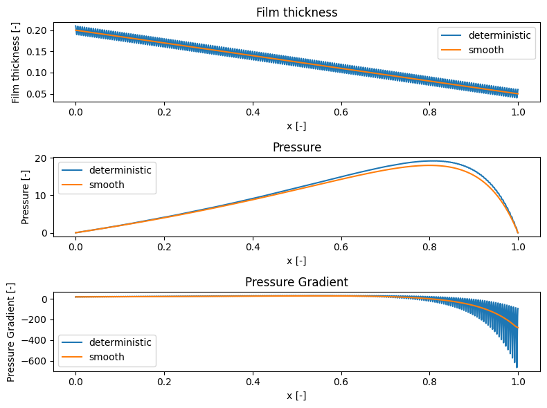
Microscale
from netgen.meshing import *

def build_micro_mesh(n, Lx):
  mesh = Mesh(dim=1)
  pids = []
  for i in range(n+1):
      pids.append (mesh.Add (MeshPoint(Pnt(i/n, 0, 0))))
  for i in range(n):
      mesh.Add(Element1D([pids[i],pids[i+1]],index=1))
  mesh.Add (Element0D( pids[0], index=1))
  mesh.Add (Element0D( pids[n], index=2))
  mesh.AddPointIdentification(pids[0],pids[n],1,2)
  mesh.SetBCName(0, "left")
  mesh.SetBCName(1, "right")
  meshout = ngsolve.Mesh(mesh)
  boundaries = meshout.GetBoundaries()
  return meshout


def Solve_microscale(zeta_i, meshm, ref, lx):
  # Unpack zeta
  h0, p0, dpdx0 = zeta_i
  ### Meshing ###
  k = 1 # Order of elements

  # Pressure gain/drop
  dpx = dpdx0 * lx # pressure increase from left to right
  # Reference pressure for point constraint - avoiding negative pressures
  pr = p0 - 0.5*dpx
  pm = pr + (dpx if dpx < 0 else 0.0)
  pconst = pr if pm >= 0.0 else (pr - pm)

  # Film thickness function
  def hg(x, h0):
    return h0 + Ah * cos(2 * pi * x*lx / lx)

  # Create a H1, order k space for the pressure field
  V_micro = Compress(H1(meshm, order=k)) # All boundaries are set to dirichlet, p = 0. Neumann conditions applied naturally in the weak form.
  V_micro.FreeDofs()[0] = False #Set the first boundary DOF as fixed - we set this to a reference value later
  V_micro.FreeDofs()[-1] = False #Set the last boundary DOF as fixed

  p = V_micro.TrialFunction()  # Pressure trial function
  v = V_micro.TestFunction()   # Pressure test function
  sol = GridFunction(V_micro)  # solution
  sol.vec[0] = pconst # Fix corner pressure value
  sol.vec[-1] = pconst + dpx

  a_micro = BilinearForm(V_micro)
  h = hg(x, h0)
  a_micro += (h**3 /  (12 * eta * lx)) * grad(p) * grad(v) * dx - (U/2) * h * grad(v) * dx
  a_micro.Assemble()

  Newton(
      a_micro,
      sol,
      freedofs=V_micro.FreeDofs(),
      maxit=200,
      maxerr=Newton_tol,
      inverse="umfpack",
      printing=False,
  )
  p_micro = GridFunction(V_micro)
  film_micro = GridFunction(V_micro)
  dpdx_micro = GridFunction(V_micro)
  p_micro.Set(sol)
  film_micro.Set(h)
  dpdx_calc = grad(p_micro)/lm
  dpdx_micro.Set(dpdx_calc)

  qx = U * h / 2 - h**3 * dpdx_micro / (12 * eta)

  Pst = Integrate(p_micro, meshm)
  Qst = Integrate(qx, meshm)
  # Qst = U * h0/2 - h0**3 * dpdx0 / (12 * eta)
  pmax = np.max(p_micro.vec.data)
  pmin = np.min(p_micro.vec.data)
  hmax = np.max(film_micro.vec.data)
  hmin = np.min(film_micro.vec.data)

  # if ref ==0:
  #   plt.plot(p_gridfunction.vec.data)
  #   plt.show()
  # if ref == 20:
  #   plt.plot(p_gridfunction.vec.data)
  #   plt.show()
  return Pst, Qst, pmax, pmin, hmax, hmin


def dP_calc(zeta_i, Pst):
  _, P, _ = zeta_i
  return Pst - P

def dQ_calc(zeta_i, Qst):
  Q_re = q_re(zeta_i)
  return Qst - Q_re
HMM Coupling
mesh_m = build_micro_mesh(Ne_m, Lx=lm)
x_vals_m = np.linspace(0, 1, Ne_m)

p_old = zeta[1,:]
p_err = 1
idx = 0
start = time.time()
while p_err > p_tol:
  print(f'Starting iteration {idx}')
  micro_results = []

  # For each set of values in zeta, run a microscale simulation
  for i in range(np.size(zeta[0,:])):
    zeta_i = zeta[:,i]
    Pst, Qst, pmax, pmin, hmax, hmin = Solve_microscale(zeta_i, mesh_m, i, lx = lm)
    micro_results.append([Pst, Qst, pmax, pmin, hmax, hmin])
  micro_results = np.asarray(micro_results)
  print(f'Total Micro calls = {i}')

  dP = dP_calc(zeta, micro_results[:,0])
  dQ = dQ_calc(zeta, micro_results[:,1])
  Q_re = q_re(zeta)

  zeta = Solve_Macroscale(mesh, hg, dQ, dP)

  p_new = zeta[1,:]
  p_err = np.linalg.norm(p_new - p_old)
  print(f'Perr: {p_err:.6f}')
  p_old = p_new
  idx += 1
print(f'HMM Time {time.time() - start}')
fig, axes = plt.subplots(2, 1, figsize=(8, 6))
axes[0].plot(micro_results[:,0]/zeta[1,:], label="Pst/P")
axes[0].set_xlabel("x [-]")
axes[0].set_ylabel("Pst/P [-]")
axes[0].set_title("Pst/P")
axes[0].legend()
axes[1].plot(micro_results[:,1]/Q_re, label="Qst/Q")
axes[1].set_xlabel("x [-]")
axes[1].set_ylabel("Qst/Q [-]")
axes[1].set_title("Qst/Q")
axes[1].legend()
plt.tight_layout()
plt.show()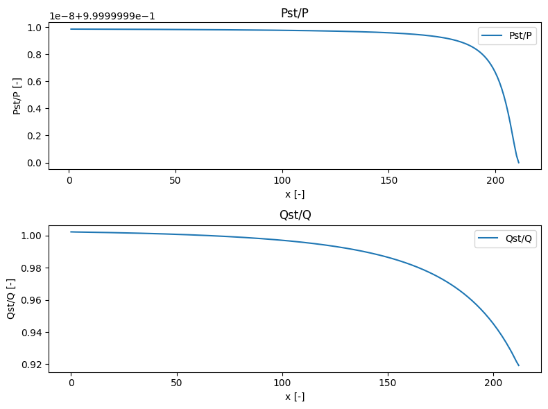
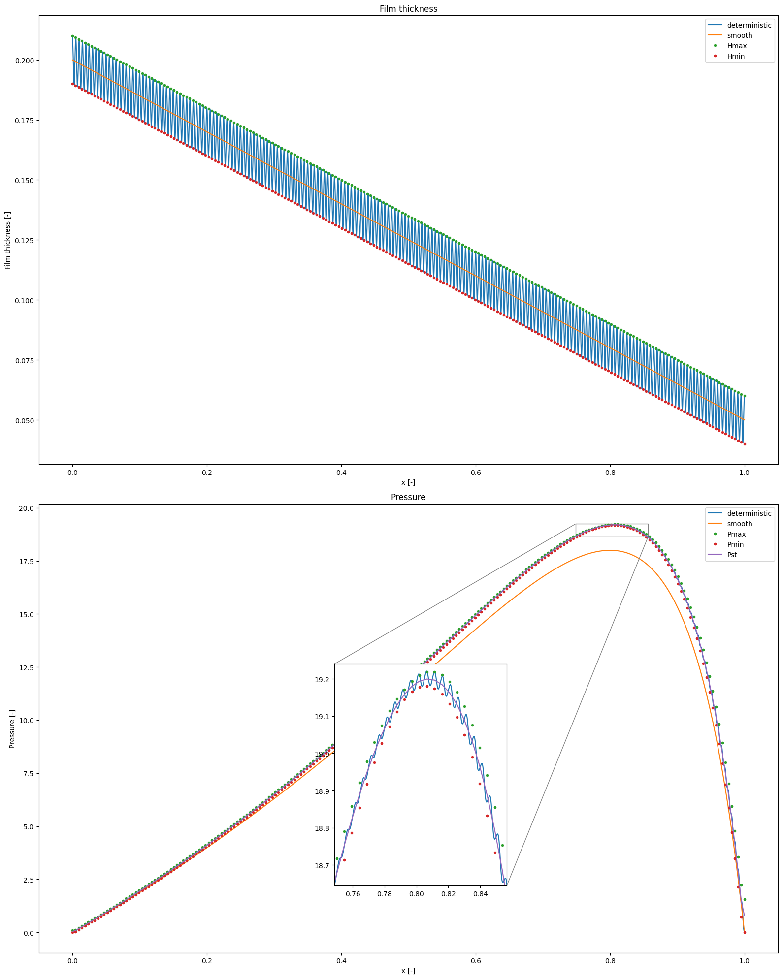
from plot_funcs import *
plot_zeta_combined2(zeta_smooth, zeta_deterministic, micro_results)